Clustering

Clustering assigns observations to groups so that points in the same cluster are more similar to each other than to points in other clusters. It is unsupervised learning and appears in exploratory analysis, customer segmentation, anomaly detection, and document organization.

SMILE’s smile.clustering package ships partitional (K-Means family), density-based (DBSCAN, HDBSCAN, DENCLUE, MEC), spectral, hierarchical, and text-oriented (SIB) algorithms. Each algorithm is a static factory that returns a rich result object with labels, optional centroids, and usually predict.

Prefer clustering when you need structure without labeled targets. Choose K-Means / K-Modes when k is known and clusters are roughly convex; X-Means / G-Means when k is unknown but roughly spherical; DBSCAN / HDBSCAN for arbitrary shapes and noise; hierarchical methods when you want a full dendrogram.

Core Abstractions

Clustering Interface and Options

Clustering defines the shared outlier sentinel and the common Options record used by most partitioning algorithms. Noise / outlier points are labeled Clustering.OUTLIER (Integer.MAX_VALUE).

Hyperparameters are fields of the nested Clustering.Options record. Pass an Options instance to fit, or a java.util.Properties map using the keys below (Options.toProperties() / Options.of(props) round-trip). Convenience constructor new Clustering.Options(k, maxIter) uses tol = 1E-4 and no controller.

k smile.clustering.k: Number of clusters (≥ 2). Default 2.
maxIter smile.clustering.iterations: Maximum iterations (> 0). Default 100.
tol smile.clustering.tolerance: Convergence tolerance (≥ 0). Default 1E-4.
controller: Optional IterativeAlgorithmController<AlgoStatus>; pass null to disable.

Partitioning

Partitioning is the base class for density-based algorithms (DBSCAN, HDBSCAN, MEC, DENCLUE) that do not produce centroids. It stores k() — the number of real clusters (excluding the outlier pseudo-cluster) — and group() labels, where noise carries Clustering.OUTLIER.

CentroidClustering

CentroidClustering<T, U> is the record returned by centroid-based algorithms. T is the centroid type and U is the observation type (usually both double[]; SIB uses different types). It implements Comparable by total distortion so Clustering.run can pick the best restart.

Method	Returns	Description
`k()`	`int`	Number of clusters
`centers()`	`T[]`	Cluster centroids / medoids
`center(i)`	`T`	Centroid of cluster `i`
`group()`	`int[]`	Per-point cluster labels
`group(i)`	`int`	Label of data point `i`
`proximity(i)`	`double`	Squared distance of point `i` to its centroid
`size(i)`	`int`	Number of points in cluster `i`
`distortions()`	`double[]`	Average squared distance per cluster + overall
`distortion()`	`double`	Overall average squared distance (WCSS / n)
`radius(i)`	`double`	RMS radius of cluster `i`: `sqrt(distortions[i])`
`predict(x)`	`int`	Assign a new point to the nearest centroid
`name()`	`String`	Algorithm name
`toString()`	`String`	Formatted cluster summary table

K-Means++ seeding is used internally by every centroid algorithm. Helpers CentroidClustering.init and CentroidClustering.seeds are also available for custom initialization.

import smile.clustering.KMeans;
import smile.datasets.GaussianMixture;
import smile.math.MathEx;

MathEx.setSeed(19650218);
var data = GaussianMixture.generate().x();
var model = KMeans.fit(data, 4, 100);
System.out.println(model);
System.out.printf("Distortion: %.4f%n", model.distortion());
System.out.printf("Cluster 0 RMS radius: %.4f%n", model.radius(0));
int label = model.predict(data[0]);
System.out.println("First point label = " + label);

import smile.clustering.KMeans
import smile.datasets.GaussianMixture
import smile.math.MathEx

MathEx.setSeed(19650218)
val data = GaussianMixture.generate.x
val model = KMeans.fit(data, 4, 100)
println(model)
println(f"Distortion: ${model.distortion}%.4f")
println(f"Cluster 0 RMS radius: ${model.radius(0)}%.4f")
println("First point label = " + model.predict(data(0)))

import smile.clustering.KMeans
import smile.datasets.GaussianMixture
import smile.math.MathEx

MathEx.setSeed(19650218)
val data = GaussianMixture.generate().x()
val model = KMeans.fit(data, 4, 100)
println(model)
println("Distortion: %.4f".format(model.distortion()))
println("Cluster 0 RMS radius: %.4f".format(model.radius(0)))
println("First point label = ${model.predict(data[0])}")

K-Means

Lloyd’s algorithm with K-Means++ initialization and BBD-tree acceleration (Kanungo et al.). The BBD-tree speeds assignment from O(nkd) toward O(n log k · d). Missing-value data is supported via KMeans.lloyd.

Default choice for numerical vectors when k is known — fast and memory-efficient even for large n.

The examples in this section (and in CLARANS, X-Means, G-Means, Deterministic Annealing, DENCLUE, MEC, and Hierarchical Clustering below) use rem.txt: 1,800 points from six 2-D Gaussian distributions — a clean mixture where centroid-based methods work well.

KMeans.fit(data, k, maxIter): Quick form returning CentroidClustering<double[], double[]>.
KMeans.fit(data, options): Full control via Clustering.Options.
KMeans.fit(bbd, data, options): Reuse a pre-built BBDTree across runs.
KMeans.lloyd(data, k, maxIter): Lloyd updates that tolerate NaN missing values.

import smile.clustering.BBDTree;
import smile.clustering.Clustering;
import smile.clustering.KMeans;
import smile.io.Read;
import smile.math.MathEx;
import org.apache.commons.csv.CSVFormat;

MathEx.setSeed(19650218);
double[][] data = Read.csv("data/clustering/rem.txt",
    CSVFormat.DEFAULT.withDelimiter(' ')).toArray();

var model = Clustering.run(20, () -> KMeans.fit(data, 6, 100));
System.out.println(model);

var bbd = new BBDTree(data);
var opts = new Clustering.Options(6, 100, 1E-4, null);
var again = KMeans.fit(bbd, data, opts);
System.out.printf("BBD distortion: %.4f%n", again.distortion());
System.out.printf("Best of 20: %.4f%n", model.distortion());

import smile.clustering.{BBDTree, Clustering, KMeans}
import smile.math.MathEx
import smile.read

MathEx.setSeed(19650218)
val data = read.csv("data/clustering/rem.txt",
  header = false, delimiter = " ").toArray
val model = Clustering.run(20, () => KMeans.fit(data, 6, 100))
println(model)

val bbd = new BBDTree(data)
val opts = new Clustering.Options(6, 100, 1E-4, null)
val again = KMeans.fit(bbd, data, opts)
println(f"BBD distortion: ${again.distortion}%.4f")
println(f"Best of 20: ${model.distortion}%.4f")

import smile.clustering.BBDTree
import smile.clustering.Clustering
import smile.clustering.KMeans
import smile.io.Read
import smile.math.MathEx
import org.apache.commons.csv.CSVFormat

MathEx.setSeed(19650218)
val data = Read.csv("data/clustering/rem.txt",
    CSVFormat.DEFAULT.withDelimiter(' ')).toArray()
val model = Clustering.run(20) { KMeans.fit(data, 6, 100) }
println(model)

val bbd = BBDTree(data)
val opts = Clustering.Options(6, 100, 1E-4, null)
val again = KMeans.fit(bbd, data, opts)
println("BBD distortion: %.4f".format(again.distortion()))
println("Best of 20: %.4f".format(model.distortion()))

Centroid methods struggle when clusters are long and thin rather than roughly spherical. The elongate.txt data (300 points) are two parallel diagonal strips. K-Means minimizes within-cluster sum of squares with Euclidean Voronoi cells, so points at the far ends of a strip are often closer to the other strip’s centroid than to their own. With k = 2 it typically cuts both strips crosswise instead of recovering the two longitudinal clusters — prefer density-based or spectral methods for shapes like this.

import smile.clustering.Clustering;
import smile.clustering.KMeans;
import smile.io.Read;
import smile.math.MathEx;
import org.apache.commons.csv.CSVFormat;

MathEx.setSeed(19650218);
double[][] data = Read.csv("data/clustering/elongate.txt",
    CSVFormat.DEFAULT.withDelimiter('\t')).toArray();
var model = Clustering.run(20, () -> KMeans.fit(data, 2, 100));
System.out.println(model);
System.out.printf("Distortion: %.4f%n", model.distortion());

import smile.clustering.{Clustering, KMeans}
import smile.math.MathEx
import smile.read

MathEx.setSeed(19650218)
val data = read.csv("data/clustering/elongate.txt",
  header = false, delimiter = "\t").toArray
val model = Clustering.run(20, () => KMeans.fit(data, 2, 100))
println(model)
println(f"Distortion: ${model.distortion}%.4f")

import smile.clustering.Clustering
import smile.clustering.KMeans
import smile.io.Read
import smile.math.MathEx
import org.apache.commons.csv.CSVFormat

MathEx.setSeed(19650218)
val data = Read.csv("data/clustering/elongate.txt",
    CSVFormat.DEFAULT.withDelimiter('\t')).toArray()
val model = Clustering.run(20) { KMeans.fit(data, 2, 100) }
println(model)
println("Distortion: %.4f".format(model.distortion()))

K-Medoids (CLARANS)

CLARANS (Clustering Large Applications based on RANdomized Search). Unlike K-Means, medoids are always actual data points. Use when centers must be real observations, when you need a custom Distance<T> on arbitrary objects, or when outliers would distort Euclidean centroids.

k: Number of clusters.
maxIter: Mapped to numLocal — number of local-minima searches (capped at 3; 2 is usually best).
tol: Ratio for maxNeighbor = tol * k * (n - k) (default 0.0125).

import smile.clustering.Clustering;
import smile.clustering.KMedoids;
import smile.io.Read;
import smile.math.MathEx;
import smile.math.distance.EuclideanDistance;
import org.apache.commons.csv.CSVFormat;

MathEx.setSeed(19650218);
double[][] data = Read.csv("data/clustering/rem.txt",
    CSVFormat.DEFAULT.withDelimiter(' ')).toArray();
var model = Clustering.run(20,
    () -> KMedoids.fit(data, new EuclideanDistance(), 6));
System.out.println(model);
System.out.printf("Distortion = %.4f%n", model.distortion());

import smile.clustering.{Clustering, KMedoids}
import smile.math.MathEx
import smile.math.distance.EuclideanDistance
import smile.read

MathEx.setSeed(19650218)
val data = read.csv("data/clustering/rem.txt",
  header = false, delimiter = " ").toArray
val model = Clustering.run(20,
  () => KMedoids.fit(data, new EuclideanDistance, 6))
println(model)
println(f"Distortion = ${model.distortion}%.4f")

import smile.clustering.Clustering
import smile.clustering.KMedoids
import smile.io.Read
import smile.math.MathEx
import smile.math.distance.EuclideanDistance
import org.apache.commons.csv.CSVFormat

MathEx.setSeed(19650218)
val data = Read.csv("data/clustering/rem.txt",
    CSVFormat.DEFAULT.withDelimiter(' ')).toArray()
val model = Clustering.run(20) {
    KMedoids.fit(data, EuclideanDistance(), 6)
}
println(model)
println("Distortion = %.4f".format(model.distortion()))

K-Modes

Categorical analogue of K-Means. Centroids are per-column modes (most frequent category), and distances are Hamming distances on integer-coded categorical features. Use for purely categorical or mixed-integer data where Euclidean distance is meaningless.

KModes.fit(int[][] data, k, maxIter): Quick form returning CentroidClustering<int[], int[]>.
KModes.fit(data, options): Full control via Clustering.Options.

import smile.clustering.KModes;
import smile.datasets.WeatherNominal;
import smile.math.MathEx;

MathEx.setSeed(19650218);
var weather = new WeatherNominal();
double[][] level = weather.level();
int[][] data = new int[level.length][level[0].length];
for (int i = 0; i < level.length; i++) {
    for (int j = 0; j < level[i].length; j++) {
        data[i][j] = (int) level[i][j];
    }
}

var model = KModes.fit(data, 2, 10);
System.out.println(model);
System.out.println("Mode of cluster 0: " +
    java.util.Arrays.toString(model.center(0)));
System.out.println("Predict: " + model.predict(data[0]));

import smile.clustering._
import smile.datasets.WeatherNominal
import smile.math.MathEx

MathEx.setSeed(19650218)
val weather = new WeatherNominal
val level = weather.level
val data = level.map(_.map(_.toInt))
val model = kmodes(data, 2, maxIter = 10)
println(model)
println("Mode of cluster 0: " + model.center(0).mkString("[", ", ", "]"))
println("Predict: " + model.predict(data(0)))

import smile.clustering.kmodes
import smile.datasets.WeatherNominal
import smile.math.MathEx

MathEx.setSeed(19650218)
val weather = WeatherNominal()
val level = weather.level()
val data = Array(level.size) { i ->
    IntArray(level[i].size) { j -> level[i][j].toInt() }
}
val model = kmodes(data, 2, maxIter = 10)
println(model)
println("Mode of cluster 0: ${model.center(0).contentToString()}")
println("Predict: ${model.predict(data[0])}")

Minimal synthetic example — Gender (0/1), Color (0–2), Size (0–2):

import smile.clustering.KModes;

int[][] data = {
    {0, 0, 0}, {0, 0, 1}, {1, 2, 2}, {1, 2, 1}
};
var model = KModes.fit(data, 2, 50);
int[] mode0 = model.center(0);
int label = model.predict(new int[]{0, 0, 0});

import smile.clustering._

val data = Array(
  Array(0, 0, 0), Array(0, 0, 1), Array(1, 2, 2), Array(1, 2, 1))
val model = kmodes(data, 2, maxIter = 50)
val mode0 = model.center(0)
val label = model.predict(Array(0, 0, 0))

import smile.clustering.kmodes

val data = arrayOf(
    intArrayOf(0, 0, 0), intArrayOf(0, 0, 1),
    intArrayOf(1, 2, 2), intArrayOf(1, 2, 1)
)
val model = kmodes(data, 2, maxIter = 50)
val mode0 = model.center(0)
val label = model.predict(intArrayOf(0, 0, 0))

X-Means

Extends K-Means by automatically determining the number of clusters. Starting from one cluster, it tries to split each centroid; a split is accepted only if the BIC of the two-child model improves under a Gaussian spherical assumption. After each splitting round, centroids are refined with BBD-tree-accelerated Lloyd updates.

Use when k is unknown and the data are reasonably Gaussian-like. The BIC criterion favors spherical, balanced clusters.

import smile.clustering.XMeans;
import smile.io.Read;
import smile.math.MathEx;
import org.apache.commons.csv.CSVFormat;

MathEx.setSeed(19650218);
double[][] data = Read.csv("data/clustering/rem.txt",
    CSVFormat.DEFAULT.withDelimiter(' ')).toArray();
var model = XMeans.fit(data, 50, 100);
System.out.printf("Discovered %d clusters, distortion = %.4f%n",
    model.k(), model.distortion());

import smile.clustering.XMeans
import smile.math.MathEx
import smile.read

MathEx.setSeed(19650218)
val data = read.csv("data/clustering/rem.txt",
  header = false, delimiter = " ").toArray
val model = XMeans.fit(data, 50, 100)
println(f"Discovered ${model.k} clusters, distortion = ${model.distortion}%.4f")

import smile.clustering.XMeans
import smile.io.Read
import smile.math.MathEx
import org.apache.commons.csv.CSVFormat

MathEx.setSeed(19650218)
val data = Read.csv("data/clustering/rem.txt",
    CSVFormat.DEFAULT.withDelimiter(' ')).toArray()
val model = XMeans.fit(data, 50, 100)
println("Discovered %d clusters, distortion = %.4f"
    .format(model.k(), model.distortion()))

G-Means

Like X-Means, but uses the Anderson-Darling test instead of BIC to decide whether to split. Cluster members are projected onto the candidate split direction; if the 1-D projection is rejected as Gaussian, the split is accepted.

Prefer G-Means when you suspect non-Gaussian within-cluster distributions — it is more sensitive to multi-modality than X-Means.

import smile.clustering.GMeans;
import smile.io.Read;
import smile.math.MathEx;
import org.apache.commons.csv.CSVFormat;

MathEx.setSeed(19650218);
double[][] data = Read.csv("data/clustering/rem.txt",
    CSVFormat.DEFAULT.withDelimiter(' ')).toArray();
var model = GMeans.fit(data, 50, 100);
System.out.printf("G-Means found %d clusters%n", model.k());

import smile.clustering.GMeans
import smile.math.MathEx
import smile.read

MathEx.setSeed(19650218)
val data = read.csv("data/clustering/rem.txt",
  header = false, delimiter = " ").toArray
val model = GMeans.fit(data, 50, 100)
println(s"G-Means found ${model.k} clusters")

import smile.clustering.GMeans
import smile.io.Read
import smile.math.MathEx
import org.apache.commons.csv.CSVFormat

MathEx.setSeed(19650218)
val data = Read.csv("data/clustering/rem.txt",
    CSVFormat.DEFAULT.withDelimiter(' ')).toArray()
val model = GMeans.fit(data, 50, 100)
println("G-Means found ${model.k()} clusters")

Deterministic Annealing

A soft-EM approach that avoids local optima by annealing temperature. At high temperature all centroids converge to the global mean; as temperature decreases, pairs of centroids split when separation exceeds a threshold, growing the model up to kmax. A final hard-assignment pass produces the CentroidClustering result.

Hyperparameters are fields of the nested DeterministicAnnealing.Options record. Pass an Options instance to fit, or a java.util.Properties map using the keys below (Options.toProperties() / Options.of(props) round-trip).

kmax smile.deterministic_annealing.k: Maximum number of clusters (≥ 2). Default 2.
alpha smile.deterministic_annealing.alpha: Temperature cooling rate in (0, 1). Typical: 0.8–0.95. Default 0.9.
maxIter smile.deterministic_annealing.iterations: Maximum Lloyd iterations at each temperature. Default 100.
tol smile.deterministic_annealing.tolerance: Convergence tolerance for soft distortion. Default 1E-4.
splitTol smile.deterministic_annealing.split_tolerance: Minimum centroid separation before a split is accepted. Default 1E-2.

import smile.clustering.DeterministicAnnealing;
import smile.io.Read;
import smile.math.MathEx;
import org.apache.commons.csv.CSVFormat;

MathEx.setSeed(19650218);
double[][] data = Read.csv("data/clustering/rem.txt",
    CSVFormat.DEFAULT.withDelimiter(' ')).toArray();
var model = DeterministicAnnealing.fit(data, 12, 0.9, 100);
System.out.printf("Converged to %d clusters, distortion = %.4f%n",
    model.k(), model.distortion());

import smile.clustering.DeterministicAnnealing
import smile.math.MathEx
import smile.read

MathEx.setSeed(19650218)
val data = read.csv("data/clustering/rem.txt",
  header = false, delimiter = " ").toArray
val model = DeterministicAnnealing.fit(data, 12, 0.9, 100)
println(f"Converged to ${model.k} clusters, distortion = ${model.distortion}%.4f")

import smile.clustering.DeterministicAnnealing
import smile.io.Read
import smile.math.MathEx
import org.apache.commons.csv.CSVFormat

MathEx.setSeed(19650218)
val data = Read.csv("data/clustering/rem.txt",
    CSVFormat.DEFAULT.withDelimiter(' ')).toArray()
val model = DeterministicAnnealing.fit(data, 12, 0.9, 100)
println("Converged to %d clusters, distortion = %.4f"
    .format(model.k(), model.distortion()))

Deterministic Annealing on six Gaussians

DBSCAN

Density-Based Spatial Clustering of Applications with Noise. A point is a core point if at least minPts neighbors lie within radius ε. Dense regions reachable from a core point form a cluster; unreachable points are labeled Clustering.OUTLIER.

Discovers arbitrary shapes, does not require k, and labels noise natively. Uses a KD-tree for double[] (O(n log n)); a LinearSearch for arbitrary types. Works poorly in high dimensions.

minPts: Minimum neighbors within radius for a core point (≥ 1). Typical: 4–10.
radius: Neighborhood radius ε (> 0). Choose at the knee of a k-NN distance plot.

The example below uses the Chameleon t4.8k dataset (8,000 noisy 2-D points with irregular cluster shapes) — a standard benchmark for density-based clustering.

import java.util.Arrays;
import smile.clustering.Clustering;
import smile.clustering.DBSCAN;
import smile.io.Read;
import org.apache.commons.csv.CSVFormat;

double[][] data = Read.csv("data/clustering/chameleon/t4.8k.txt",
    CSVFormat.DEFAULT.withDelimiter(' ')).toArray();
DBSCAN<double[]> model = DBSCAN.fit(data, 20, 10);
System.out.printf("Found %d clusters%n", model.k());

long noise = Arrays.stream(model.group())
    .filter(l -> l == Clustering.OUTLIER).count();
System.out.printf("Noise points: %d%n", noise);
int label = model.predict(data[0]);
if (label == Clustering.OUTLIER) System.out.println("Noise");
else System.out.println("Cluster " + label);

import smile.clustering.{Clustering, DBSCAN}
import smile.read

val data = read.csv("data/clustering/chameleon/t4.8k.txt",
  header = false, delimiter = " ").toArray
val model = DBSCAN.fit(data, 20, 10)
println(s"Found ${model.k} clusters")
val noise = model.group.count(_ == Clustering.OUTLIER)
println(s"Noise points: $noise")
val label = model.predict(data(0))
println(if (label == Clustering.OUTLIER) "Noise" else s"Cluster $label")

import smile.clustering.Clustering
import smile.clustering.DBSCAN
import smile.io.Read
import org.apache.commons.csv.CSVFormat

val data = Read.csv("data/clustering/chameleon/t4.8k.txt",
    CSVFormat.DEFAULT.withDelimiter(' ')).toArray()
val model = DBSCAN.fit(data, 20, 10)
println("Found ${model.k()} clusters")
val noise = model.group().count { it == Clustering.OUTLIER }
println("Noise points: $noise")
val label = model.predict(data[0])
println(if (label == Clustering.OUTLIER) "Noise" else "Cluster $label")

HDBSCAN

Hierarchical DBSCAN builds a full density hierarchy (mutual-reachability MST → condensed tree) and selects stable flat clusters via a stability criterion. Unlike DBSCAN, it handles clusters of varying density without a global ε.

Pipeline: core distances from minPoints nearest neighbors → mutual-reachability graph → MST → condensed hierarchy pruned by minClusterSize.

Note: the current implementation computes full pairwise distances (O(n²) memory and time). For very large datasets consider sub-sampling.

Hyperparameters are fields of the nested HDBSCAN.Options record. Pass an Options instance to fit, or a java.util.Properties map using the keys below (Options.toProperties() / Options.of(props) round-trip). Convenience form: HDBSCAN.fit(data, minPoints, minClusterSize). Also accepts a custom Distance<T>.

minPoints: Neighborhood size for core-distance estimation. Larger = smoother density.
minClusterSize: Minimum cluster size in the condensed hierarchy. Controls granularity.

import smile.clustering.Clustering;
import smile.clustering.HDBSCAN;
import smile.io.Read;
import org.apache.commons.csv.CSVFormat;

double[][] data = Read.csv("data/clustering/chameleon/t4.8k.txt",
    CSVFormat.DEFAULT.withDelimiter(' ')).toArray();
HDBSCAN<double[]> model = HDBSCAN.fit(data, 20, 40);
System.out.printf("Found %d clusters%n", model.k());
double[] stability = model.stability();
for (int i = 0; i < model.k(); i++) {
    System.out.printf("Cluster %d stability: %.4f%n", i, stability[i]);
}
long noise = java.util.Arrays.stream(model.group())
    .filter(l -> l == Clustering.OUTLIER).count();
System.out.println("Outliers: " + noise);

import smile.clustering.{Clustering, HDBSCAN}
import smile.read

val data = read.csv("data/clustering/chameleon/t4.8k.txt",
  header = false, delimiter = " ").toArray
val model = HDBSCAN.fit(data, 20, 40)
println(s"Found ${model.k} clusters")
model.stability.zipWithIndex.foreach { case (s, i) =>
  println(f"Cluster $i stability: $s%.4f")
}
println("Outliers: " + model.group.count(_ == Clustering.OUTLIER))

import smile.clustering.Clustering
import smile.clustering.HDBSCAN
import smile.io.Read
import org.apache.commons.csv.CSVFormat

val data = Read.csv("data/clustering/chameleon/t4.8k.txt",
    CSVFormat.DEFAULT.withDelimiter(' ')).toArray()
val model = HDBSCAN.fit(data, 20, 40)
println("Found ${model.k()} clusters")
model.stability().forEachIndexed { i, s ->
    println("Cluster $i stability: %.4f".format(s))
}
val outliers = model.group().count { it == Clustering.OUTLIER }
println("Outliers: $outliers")

DENCLUE

DENsity CLUstering selects m representative sample points via K-Means (“particles”), then hill-climbs the Gaussian kernel density estimate from each training point to its local density maximum (“attractor”). DBSCAN is run on the attractors for the final assignment.

Best for smooth, continuous data with density peaks — not for high dimensions, sparse data, or uniform distributions.

Hyperparameters are fields of the nested DENCLUE.Options record. Pass an Options instance to fit, or a java.util.Properties map using the keys below (Options.toProperties() / Options.of(props) round-trip). Quick form: DENCLUE.fit(data, sigma, m). predict(x) may return Clustering.OUTLIER.

sigma smile.denclue.sigma: Gaussian kernel bandwidth. Choose so attractor count is stable across a range of sigma. Default 1.0.
m smile.denclue.m: Number of sample points for KDE (≪ n). Default 100.
minPts smile.denclue.min_points: Minimum attractor neighborhood for DBSCAN post-processing. Default 10.
tol smile.denclue.tolerance: Hill-climbing convergence tolerance. Default 1E-2.

import smile.clustering.DENCLUE;
import smile.io.Read;
import smile.math.MathEx;
import org.apache.commons.csv.CSVFormat;

MathEx.setSeed(19650218);
double[][] data = Read.csv("data/clustering/rem.txt",
    CSVFormat.DEFAULT.withDelimiter(' ')).toArray();
DENCLUE model = DENCLUE.fit(data, 1.0, 50);
System.out.printf("DENCLUE found %d clusters%n", model.k());
System.out.println("Predict first: " + model.predict(data[0]));

import smile.clustering.DENCLUE
import smile.math.MathEx
import smile.read

MathEx.setSeed(19650218)
val data = read.csv("data/clustering/rem.txt",
  header = false, delimiter = " ").toArray
val model = DENCLUE.fit(data, 1.0, 50)
println(s"DENCLUE found ${model.k} clusters")
println("Predict first: " + model.predict(data(0)))

import smile.clustering.DENCLUE
import smile.io.Read
import smile.math.MathEx
import org.apache.commons.csv.CSVFormat

MathEx.setSeed(19650218)
val data = Read.csv("data/clustering/rem.txt",
    CSVFormat.DEFAULT.withDelimiter(' ')).toArray()
val model = DENCLUE.fit(data, 1.0, 50)
println("DENCLUE found ${model.k()} clusters")
println("Predict first: ${model.predict(data[0])}")

MEC

Non-parametric Minimum Conditional Entropy Clustering minimizes H(C | x) by iteratively relabeling each point to reduce entropy in its neighborhood (Parzen density estimate). Unlike DBSCAN/DENCLUE, MEC needs a good initialization — the public MEC.fit(data, distance, k, radius) API initializes from K-Means (Euclidean double[][]) or K-Medoids (arbitrary distance).

Effective when the true cluster count is uncertain: start with a generous k; MEC may merge clusters toward lower entropy. MEC implements Comparable by entropy for use with Clustering.run.

Hyperparameters are fields of the nested MEC.Options record. Pass an Options instance to fit, or a java.util.Properties map using the keys below (Options.toProperties() / Options.of(props) round-trip). Primary API: MEC.fit(data, distance, k, radius). Full control uses MEC.fit(data, nns, group, options) with a precomputed initial partition.

k smile.mec.k: Initial number of clusters (hint; final count may be smaller). Default 2.
radius smile.mec.radius: Parzen window radius for density estimation. Default 1.0.
maxIter smile.mec.iterations: Maximum relabeling iterations. Default 500.
tol smile.mec.tolerance: Convergence tolerance. Default 1E-4.

import smile.clustering.Clustering;
import smile.clustering.MEC;
import smile.io.Read;
import smile.math.MathEx;
import smile.math.distance.EuclideanDistance;
import org.apache.commons.csv.CSVFormat;

MathEx.setSeed(19650218);
double[][] data = Read.csv("data/clustering/rem.txt",
    CSVFormat.DEFAULT.withDelimiter(' ')).toArray();
MEC<double[]> model = MEC.fit(data, new EuclideanDistance(), 20, 2.0);
System.out.printf("MEC entropy: %.4f, clusters: %d%n",
    model.entropy(), model.k());

MEC<double[]> best = Clustering.run(5,
    () -> MEC.fit(data, new EuclideanDistance(), 20, 2.0));
System.out.printf("Best entropy: %.4f%n", best.entropy());

import smile.clustering.{Clustering, MEC}
import smile.math.MathEx
import smile.math.distance.EuclideanDistance
import smile.read

MathEx.setSeed(19650218)
val data = read.csv("data/clustering/rem.txt",
  header = false, delimiter = " ").toArray
val model = MEC.fit(data, new EuclideanDistance, 20, 2.0)
println(f"MEC entropy: ${model.entropy}%.4f, clusters: ${model.k}")
val best = Clustering.run(5, () => MEC.fit(data, new EuclideanDistance, 20, 2.0))
println(f"Best entropy: ${best.entropy}%.4f")

import smile.clustering.Clustering
import smile.clustering.MEC
import smile.io.Read
import smile.math.MathEx
import smile.math.distance.EuclideanDistance
import org.apache.commons.csv.CSVFormat

MathEx.setSeed(19650218)
val data = Read.csv("data/clustering/rem.txt",
    CSVFormat.DEFAULT.withDelimiter(' ')).toArray()
val model = MEC.fit(data, EuclideanDistance(), 20, 2.0)
println("MEC entropy: %.4f, clusters: %d".format(model.entropy(), model.k()))
val best = Clustering.run(5) {
    MEC.fit(data, EuclideanDistance(), 20, 2.0)
}
println("Best entropy: %.4f".format(best.entropy()))

SIB

Sequential Information Bottleneck clusters document vectors (sparse term histograms) by minimizing Jensen-Shannon divergence between cluster centroids and member distributions. Each iteration reassigns every document to the cluster that most reduces JS divergence.

Use for text clustering (bag-of-words or TF-IDF). Input is SparseArray[] normalized so each row sums to 1. The result is CentroidClustering<double[], SparseArray> (dense centroid coordinates, sparse observations).

import smile.clustering.SIB;
import smile.util.SparseArray;

// Build normalized term-frequency vectors (each SparseArray sums to 1)
SparseArray[] docs = /* ... */;

var model = SIB.fit(docs, 5, 100);
System.out.printf("SIB JS distortion: %.4f%n", model.distortion());
int label = model.predict(docs[0]);

import smile.clustering._
import smile.util.SparseArray

// Build normalized term-frequency vectors (each SparseArray sums to 1)
val docs: Array[SparseArray] = ???

val model = sib(docs, 5, maxIter = 100)
println(f"SIB JS distortion: ${model.distortion}%.4f")
val label = model.predict(docs(0))

import smile.clustering.sib
import smile.util.SparseArray

// Build normalized term-frequency vectors (each SparseArray sums to 1)
val docs: Array<SparseArray> = TODO()

val model = sib(docs, 5, maxIter = 100)
println("SIB JS distortion: %.4f".format(model.distortion()))
val label = model.predict(docs[0])

Spectral Clustering

Builds an RBF similarity matrix, computes the normalized graph Laplacian, embeds data in the top-k eigenvectors, then runs K-Means in that embedding. Captures non-convex clusters and manifold structure.

For large n, set Nyström sample count l > 0 to approximate eigenvectors without the full n×n matrix (cost O(nl) instead of O(n²)). Sparse text path: SpectralClustering.fit(SparseIntArray[], p, Clustering.Options) builds a TF-IDF-weighted Laplacian for term-count arrays.

Hyperparameters are fields of the nested SpectralClustering.Options record. Pass an Options instance to fit, or a java.util.Properties map using the keys below (Options.toProperties() / Options.of(props) round-trip). Fit with SpectralClustering.fit(data, options). Convenience constructor new Options(k, sigma, maxIter) sets l = 0.

k smile.spectral_clustering.k: Number of clusters (≥ 2). Default 2.
l smile.spectral_clustering.l: Nyström sample count. Use 0 for exact. Must be ≥ k if > 0. Default 0.
sigma smile.spectral_clustering.sigma: RBF kernel width. Sensitive; tune on your data. Default 1.0.
maxIter smile.spectral_clustering.iterations: K-Means iterations in embedding space. Default 100.
tol smile.spectral_clustering.tolerance: K-Means convergence tolerance. Default 1E-4.

The example uses sincos.txt (300 points): two interlocking crescent “moons.” They are not linearly separable and are poorly suited to spherical centroids — K-Means tends to cut each arc in half. With a suitable RBF width, spectral clustering embeds the graph connectivity so the two manifolds separate cleanly.

import smile.clustering.SpectralClustering;
import smile.io.Read;
import smile.math.MathEx;
import org.apache.commons.csv.CSVFormat;

MathEx.setSeed(19650218);
double[][] data = Read.csv("data/clustering/sincos.txt",
    CSVFormat.DEFAULT.withDelimiter('\t')).toArray();
var opts = new SpectralClustering.Options(2, 0.2, 100);
var model = SpectralClustering.fit(data, opts);
System.out.printf("Spectral clustering: %d clusters, distortion = %.4f%n",
    model.k(), model.distortion());

import smile.clustering.SpectralClustering
import smile.math.MathEx
import smile.read

MathEx.setSeed(19650218)
val data = read.csv("data/clustering/sincos.txt",
  header = false, delimiter = "\t").toArray
val opts = new SpectralClustering.Options(2, 0.2, 100)
val model = SpectralClustering.fit(data, opts)
println(f"Spectral clustering: ${model.k} clusters, distortion = ${model.distortion}%.4f")

import smile.clustering.SpectralClustering
import smile.io.Read
import smile.math.MathEx
import org.apache.commons.csv.CSVFormat

MathEx.setSeed(19650218)
val data = Read.csv("data/clustering/sincos.txt",
    CSVFormat.DEFAULT.withDelimiter('\t')).toArray()
val opts = SpectralClustering.Options(2, 0.2, 100)
val model = SpectralClustering.fit(data, opts)
println("Spectral clustering: %d clusters, distortion = %.4f"
    .format(model.k(), model.distortion()))

Hierarchical Clustering

Agglomerative bottom-up clustering: each observation starts alone; pairs merge greedily by the chosen linkage until one cluster remains. The full dendrogram can be cut by cluster count or merge height.

Use when you want to explore hierarchy without committing to a fixed k, on small-to-medium data (O(n²) / O(n² log n)), or when the dendrogram itself is insightful. Linkage stores distances as float and supports at most 65 535 observations.

HierarchicalClustering.fit(linkage): Build the full dendrogram from any Linkage.
partition(k): Cut into k clusters.
partition(h): Cut by merge height. Height array must be monotonically non-decreasing.
tree() / height(): (n−1)×2 merge table and merge heights.

Linkage Methods

All linkage classes live in smile.clustering.linkage and implement Linkage. Build from a data matrix (WardLinkage.of(data)) or a pre-computed proximity matrix.

Class	Update	Notes
`SingleLinkage`	min(d(a,x), d(b,x))	Chaining effect; sensitive to outliers
`CompleteLinkage`	max(d(a,x), d(b,x))	Compact, balanced clusters
`UPGMALinkage`	size-weighted average	UPGMA; good general-purpose choice
`WPGMALinkage`	unweighted average	WPGMA; ignores cluster sizes
`UPGMCLinkage`	centroid of centroids (squared)	Stored as squared distance; height sqrt’d at output
`WPGMCLinkage`	midpoint (squared)	Stored as squared distance; height sqrt’d at output
`WardLinkage`	minimizes within-cluster variance	Best cluster quality; similar to K-Means

import smile.clustering.HierarchicalClustering;
import smile.clustering.linkage.CompleteLinkage;
import smile.io.Read;
import org.apache.commons.csv.CSVFormat;

double[][] data = Read.csv("data/clustering/rem.txt",
    CSVFormat.DEFAULT.withDelimiter(' ')).toArray();
var model = HierarchicalClustering.fit(CompleteLinkage.of(data));
int[] labels = model.partition(6);
System.out.println("Cut into 6: first labels = "
    + java.util.Arrays.toString(
        java.util.Arrays.copyOf(labels, 5)));
double[] heights = model.height();
System.out.printf("Last merge height: %.4f%n",
    heights[heights.length - 1]);

import smile.clustering.HierarchicalClustering
import smile.clustering.linkage.CompleteLinkage
import smile.read

val data = read.csv("data/clustering/rem.txt",
  header = false, delimiter = " ").toArray
val model = HierarchicalClustering.fit(CompleteLinkage.of(data))
val labels = model.partition(6)
println("Cut into 6: first labels = " + labels.take(5).mkString("[", ", ", "]"))
val heights = model.height
println(f"Last merge height: ${heights.last}%.4f")

import smile.clustering.hclust
import smile.io.Read
import org.apache.commons.csv.CSVFormat

val data = Read.csv("data/clustering/rem.txt",
    CSVFormat.DEFAULT.withDelimiter(' ')).toArray()
val model = hclust(data, "complete")
val labels = model.partition(6)
println("Cut into 6: first labels = ${labels.take(5).contentToString()}")
val heights = model.height()
println("Last merge height: %.4f".format(heights.last()))

Single linkage shines on connectivity-defined shapes. On sincos.txt (the same interlocking moons as in Spectral Clustering), chaining along nearest neighbors recovers each crescent; a large gap in the dendrogram marks the cut into two clusters. Centroid methods typically fail here.

import smile.clustering.HierarchicalClustering;
import smile.clustering.linkage.SingleLinkage;
import smile.io.Read;
import org.apache.commons.csv.CSVFormat;

double[][] data = Read.csv("data/clustering/sincos.txt",
    CSVFormat.DEFAULT.withDelimiter('\t')).toArray();
var model = HierarchicalClustering.fit(SingleLinkage.of(data));
int[] labels = model.partition(2);
System.out.println("Cut into 2: first labels = "
    + java.util.Arrays.toString(
        java.util.Arrays.copyOf(labels, 5)));
double[] heights = model.height();
System.out.printf("Last merge height: %.4f%n",
    heights[heights.length - 1]);

import smile.clustering.HierarchicalClustering
import smile.clustering.linkage.SingleLinkage
import smile.read

val data = read.csv("data/clustering/sincos.txt",
  header = false, delimiter = "\t").toArray
val model = HierarchicalClustering.fit(SingleLinkage.of(data))
val labels = model.partition(2)
println("Cut into 2: first labels = " + labels.take(5).mkString("[", ", ", "]"))
val heights = model.height
println(f"Last merge height: ${heights.last}%.4f")

import smile.clustering.hclust
import smile.io.Read
import org.apache.commons.csv.CSVFormat

val data = Read.csv("data/clustering/sincos.txt",
    CSVFormat.DEFAULT.withDelimiter('\t')).toArray()
val model = hclust(data, "single")
val labels = model.partition(2)
println("Cut into 2: first labels = ${labels.take(5).contentToString()}")
val heights = model.height()
println("Last merge height: %.4f".format(heights.last()))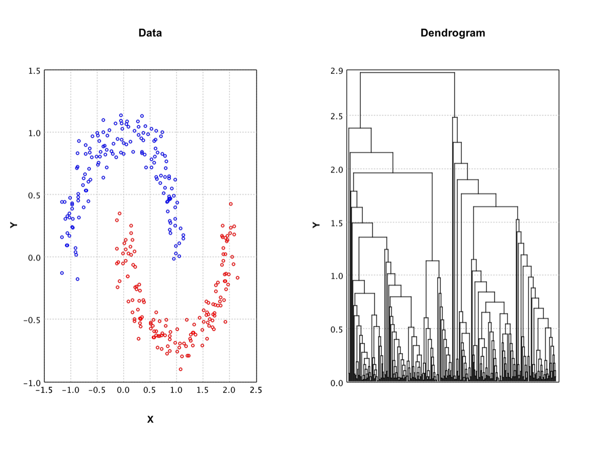

Single-linkage hierarchical clustering on two moons

Linkage Selection

Goal	Recommended linkage
Compact spherical clusters	`WardLinkage`
Long chains or arbitrary shape	`SingleLinkage`
Balanced clusters, moderate sensitivity	`CompleteLinkage`
Robust average (bioinformatics)	`UPGMALinkage`

Running Multiple Trials

Algorithms with random initialization (K-Means, K-Medoids, K-Modes, MEC, …) may converge to different local optima. Clustering.run(n, supplier) repeats the fit n times and returns the best result by compareTo (distortion for CentroidClustering, entropy for MEC). Throws if runs ≤ 0.

import smile.clustering.Clustering;
import smile.clustering.KMeans;
import smile.datasets.GaussianMixture;
import smile.math.MathEx;

MathEx.setSeed(19650218);
double[][] data = GaussianMixture.generate().x();
var best = Clustering.run(10, () -> KMeans.fit(data, 4, 100));
System.out.printf("Best distortion: %.4f%n", best.distortion());

import smile.clustering.{Clustering, KMeans}
import smile.datasets.GaussianMixture
import smile.math.MathEx

MathEx.setSeed(19650218)
val data = GaussianMixture.generate.x
val best = Clustering.run(10, () => KMeans.fit(data, 4, 100))
println(f"Best distortion: ${best.distortion}%.4f")

import smile.clustering.Clustering
import smile.clustering.KMeans
import smile.datasets.GaussianMixture
import smile.math.MathEx

MathEx.setSeed(19650218)
val data = GaussianMixture.generate().x()
val best = Clustering.run(10) { KMeans.fit(data, 4, 100) }
println("Best distortion: %.4f".format(best.distortion()))

Algorithm Comparison

Algorithm	k required	Outliers	Arbitrary shape	Distance	Data type	Scalability
K-Means	Yes	No	No (convex)	Euclidean	`double[]`	O(nkd·iter) fast
K-Medoids	Yes	Partial	No (convex)	Any	Any	O(n²k)
K-Modes	Yes	No	No (convex)	Hamming	`int[]` categorical	O(nkd·iter)
X-Means	Upper bound	No	No (spherical)	Euclidean	`double[]`	O(nkd·iter)
G-Means	Upper bound	No	No	Euclidean	`double[]`	O(nkd·iter)
Det. Annealing	Upper bound	No	No	Euclidean	`double[]`	Slow (multi-temperature)
DBSCAN	No	Yes	Yes	Any	Any (KD-tree for `double[]`)	O(n log n) w/ index
HDBSCAN	No	Yes	Yes	Any	Any	O(n²) current impl.
DENCLUE	No	Yes	Yes (density)	Euclidean	`double[]`	O(nm·iter)
MEC	Initial k	Yes	Yes (density)	Any	Any	O(n·radius·iter)
SIB	Yes	No	No	Jensen-Shannon	`SparseArray` text	O(nkd·iter)
Spectral	Yes	No	Yes (manifold)	RBF kernel	`double[]`	O(n²) or O(nl) w/ Nyström
Hierarchical	Post-hoc	Partial	Yes	Any	Any (float prox.)	O(n² log n), ≤ 65 535 pts

Common Patterns

Choosing k

Unknown k: X-Means or G-Means for Gaussian-like data; DBSCAN or HDBSCAN for density-based / irregular clusters; MEC when you have an initial partition.

Elbow: run K-Means for k = 2…K, plot model.distortion() vs. k, pick the elbow.

Silhouette: compare k values with smile.validation.metric.Silhouette.

Handling Outliers

DBSCAN, HDBSCAN, DENCLUE, and MEC label noise with Clustering.OUTLIER. Centroid methods are sensitive to outliers — consider removing noise with DBSCAN before K-Means.

Reproducibility

Randomized algorithms respect SMILE’s global RNG. Call MathEx.setSeed(…) before every fit for repeatable results.

import smile.math.MathEx;
MathEx.setSeed(42);

import smile.math.MathEx
MathEx.setSeed(42)

import smile.math.MathEx
MathEx.setSeed(42)

Serialization

Most models implement java.io.Serializable. Persist with smile.io.Write.object / smile.io.Read.object. Dedicated Options records also round-trip through java.util.Properties.

import smile.io.*;
import smile.clustering.CentroidClustering;
import java.nio.file.Path;

Path file = Write.object(model);
@SuppressWarnings("unchecked")
var loaded = (CentroidClustering<double[], double[]>) Read.object(file);

← Unified Training Vector Quantization →